
A geo experiment settles the question that attribution and MMM cannot settle on their own: would these sales have happened without this channel? You change spend in some regions, leave the others alone, and compare the treated regions with a forecast built from the untouched ones. It works for branch sales, TV, outdoor and any ad platform, because all it needs is spend and your own KPI by region and week. The hard part is power: with about 20 usable regions in Kazakhstan and lifts of a few percent, a test designed without a power analysis comes back "not significant" and burns the budget.
This is part three of a four-part series. The MMM overview explains what the model estimates, Google Meridian in practice shows how to build one, and Meridian vs Robyn vs PyMC-Marketing compares the libraries. This article is about the experiments that keep those models honest.
Why experiments: correlation is not incrementality
An MMM is a regression on history. Google's measurement playbook says it plainly: because MMM rests on correlations, its accuracy depends on the scale, timing and variation of past spend, and it struggles most with small channels, always-on channels and pull media such as search.¹ If brand search spend rises every time demand rises, the model cannot tell which one caused the other. Attribution has the opposite blind spot: it counts who clicked before converting, not who would have converted anyway.
An experiment breaks the correlation by changing spend on purpose, in a part of the market you choose, while the rest of the market serves as the comparison. In a geo experiment the units are regions: non-overlapping areas that the ad platforms can target separately and in which you can count the KPI separately.² Because the test needs only aggregates (spend and KPI per region per day or week), no user-level data is involved, which is why Google describes geo experiments as a privacy-conscious way to measure media.³
What a geo test estimates
Every number a geo test produces is a comparison with a counterfactual: what the treated regions would have done without the change. Nobody observes that directly, so the method's whole job is to forecast it from the regions that were not touched.
Here is the actual KPI of the treatment group in week t, is the counterfactual forecast for the same week, and Δ is the incremental KPI summed over the test weeks. GeoX calls this the average treatment effect on the treated at the geo level; from a user's point of view it is an intention-to-treat effect, because not everyone in a treated region sees the ads.³
is the incremental spend, so iROAS (incremental return on ad spend) is incremental revenue per extra dollar, and lift is the incremental KPI as a share of the counterfactual. When the KPI is not revenue (applications, issued policies), the same ratio becomes incremental conversions per dollar, or its inverse, cost per incremental conversion. GeoX reports it as iCPD, incremental conversions per dollar, which equals iROAS when the KPI is revenue.⁴
When user-level lift tests are not enough
Platform conversion lift studies randomise users, and within their scope they are cleaner and cheaper than a geo test. The scope is the problem:
| User-level conversion lift | Geo experiment | |
|---|---|---|
| What is randomised | Users or cookies inside one platform | Regions |
| KPI | Conversions the platform can track | Your own backend KPI, online and offline |
| Channels | One platform at a time | Any channel you can buy by region: search, social, video, OOH, regional TV |
| Comparable across platforms | No: each platform tests its own audience and its own conversion definition | Yes: same KPI, same method |
| Scale needed | Feasible for smaller campaigns | Needs volume: enough regions, spend and KPI |
Google's playbook makes the same split: user-based lift is subject to tracking gaps (ITP, in-app browsers), while open-source geo experiments represent all realised conversions but are resource-intensive and noisier, so they suit bigger channels.¹ Meta's GeoLift documentation notes that its own lift studies depend on access to online signals such as pixels, APIs and SDKs.⁵ For a bank, insurer or retailer whose sale closes in a branch, a call centre or a back office, the conversion the platform never sees is the whole question. If that is your situation, the offline branch attribution article shows how to get those conversions into data in the first place.
Three designs: holdback, go-dark, heavy-up
Meridian GeoX, Google's open-source geo-experiment framework, names three intervention types.⁶ They answer different budget questions, and they enter an MMM differently, so pick the design from the question, not from habit.
- New spend vs none. Holdback. Treatment regions get the new channel, campaign or format; control regions get none. Use it to validate a net-new channel before scaling it. It measures the average return of the whole spend against zero.
- Live spend switched off. Go-dark. Spend in treatment regions is turned off; control regions keep business as usual. Use it to prove what a live channel is worth: the sales you would lose without it. The measured effect is negative and the analysis flips its sign. Also measured against zero spend.
- Extra spend on top. Heavy-up. Treatment regions get business as usual plus X%; control regions stay at business as usual. Use it to price the next budget increment, or when current spend is too small to power a go-dark. It measures a marginal return, not the average one.
GeoX also distinguishes single-cell tests (one treatment group against one control) from multi-cell tests (several treatment groups sharing one control). Its documentation calls single-cell the more robust option, because all the statistical power goes into one comparison, while multi-cell needs significantly more regions and budget and ends up with a higher minimum detectable effect.⁶ With about 20 regions, I would not run a multi-cell test.
Decide the question first. Holdback and go-dark answer "is this channel worth its total budget?", the average return. A heavy-up answers "should the next dollar go here?", the marginal return. On a saturating response curve the two can differ a lot, and, as shown below, they also feed an MMM through different doors.
Randomised, stratified, paired or matched
Once the intervention is fixed, decide which regions get it.
- Full randomisation. A coin flip per region protects against known and unknown differences between regions, but only when there are many of them. With few regions a coin flip can easily put all the large cities on one side.⁷
- Stratified randomisation. Group similar regions first, then randomise within each group. Vaver and Koehler found that grouping geos by size before assignment can shrink the confidence interval of ROAS by 10% or more.² GeoX does this by default: it describes each region's KPI series by its mean, coefficient of variation, trend slope, lag-1 autocorrelation and dynamic time warping distance, clusters the regions into four strata with k-means, and randomises within strata.³ Candidate designs survive only if the counterfactual fits well out of sample (R² of at least 0.8 by default) and an A/A test on held-out pre-period data shows no bias; the survivors are ranked by minimum detectable effect.⁴
- Paired randomisation. Sort regions by size, pair neighbours, flip a coin inside each pair. This is the design Trimmed Match is built for,⁸ and Kerman et al. use the same pairing in their power analysis for TBR.⁷
- Matched markets. Hand-pick one or a few test markets and comparable controls. It is cheap and practical, but Kerman et al. are explicit that it lacks randomisation's protection against hidden biases.⁷ GeoLift's market selection is a power-driven version of this: it ranks candidate sets of test markets by simulated power and reports the minimum detectable effect for each.⁵
My rule: randomise, stratified or paired, whenever the region count allows it, and fall back to matched markets with a synthetic control only when there are very few regions or when one or two of them cannot go into treatment at random.
Reading a geo test with time-based regression
Time-based regression (TBR), published by Kerman, Wang and Vaver in 2017, is the workhorse of Google's geo testing and the primary method in GeoX.⁷ ³ The KPI is first summed (or averaged) across regions into one series per group per day or week. On the pre-period, the treatment series is regressed on the control series:
and are the treatment and control KPI in week t, a absorbs the level difference between the groups, b captures how the treatment group moves with the control group, and is the residual. GeoX can constrain b to be non-negative and makes no distributional assumption about the residual, relying on placebo-based inference instead.³ In the test period, the fitted line turns the control group's actual numbers into the treatment group's counterfactual:
is the effect in test week t, Δ(t) is the cumulative effect up to week t, and iROAS(t) divides the cumulative incremental response by the cumulative incremental cost. Kerman et al. recommend watching the cumulative curve: when it keeps rising after the spend change ends, the effect is lagged and the analysis needs a cool-down period; when it flattens, it does not.⁷ TBR works with as few as one test and one control region, which is why it also serves matched-market tests.⁷
Worked example: a four-week heavy-up
The numbers below are synthetic and come from the generator behind every chart in this series. Twelve weeks of revenue for a control group and a treatment group: eight pre-test weeks, then four test weeks during which the treatment group got a heavy-up of $20k extra spend in total. An ordinary least squares fit on the eight pre-test weeks gives a = 39.69 and b = 0.4561, so the counterfactual for week 9 is 39.69 + 0.4561 × 432.0 = 236.7.
| Week | Period | Control, $k | Treatment, $k | Counterfactual a + b × control, $k | Effect φ, $k |
|---|---|---|---|---|---|
| 1 | Pre-test | 395.5 | 218.6 | - | - |
| 2 | Pre-test | 413.0 | 228.7 | - | - |
| 3 | Pre-test | 438.6 | 239.9 | - | - |
| 4 | Pre-test | 442.9 | 239.0 | - | - |
| 5 | Pre-test | 449.0 | 242.3 | - | - |
| 6 | Pre-test | 439.4 | 242.4 | - | - |
| 7 | Pre-test | 439.3 | 242.2 | - | - |
| 8 | Pre-test | 424.6 | 234.6 | - | - |
| 9 | Heavy-up | 432.0 | 245.3 | 236.7 | 8.6 |
| 10 | Heavy-up | 433.6 | 245.9 | 237.5 | 8.4 |
| 11 | Heavy-up | 437.6 | 249.1 | 239.3 | 9.8 |
| 12 | Heavy-up | 444.8 | 249.0 | 242.6 | 6.4 |
| Test total | 989.3 | 956.1 | 33.2 |
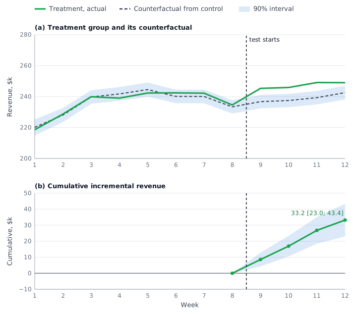
The read-out:
- Incremental revenue Δ = 8.6 + 8.4 + 9.8 + 6.4 = $33.2k.
- iROAS = 33.2 / 20 = 1.66: each extra dollar returned $1.66 of revenue on top of what would have happened anyway.
- Lift = 33.2 / 956.1 = 3.5% over the counterfactual.
Now the honest part. The generator injected a true effect of 9 + 11 + 10 + 8 = $38k, so the point estimate misses the truth by $4.8k, about 13% (4.8 / 38). Nothing is broken: eight weeks are simply not enough to pin down a and b. The generator's true values are a = 20 and b = 0.5; the fit found 39.69 and 0.4561, two errors that partly cancel inside the pre-period and do not cancel exactly in the test weeks. That is why a geo test is reported with an interval. Kerman et al. give the variance of the cumulative effect after T test weeks:⁷
The sums run over the T test weeks and σ is the residual standard deviation. The first three terms are the uncertainty of the fitted line, which shrinks as the pre-period grows; the last term is the fresh noise of the test weeks, which grows with T. With σ estimated from n pre-period weeks, the interval uses a t-distribution with n - 2 degrees of freedom. Applied to the twelve weeks in the table, the standard error of Δ is $5.24k and , so the 90% interval is 33.2 ± 10.2, from $23.0k to $43.4k. Dividing by the known $20k of extra spend, iROAS lies between 1.15 and 2.17. The true $38k sits inside the interval; the point estimate on its own would have hidden how wide the honest answer is.
Whether that answer is good enough depends on the decision. If the channel needs an iROAS above 1.0 to pay for itself on margin, this test says yes. If the bar is 2.0, it cannot tell you, and running it longer or with more spend would have been the right call. Also note that the example breaks the rules on purpose to keep the chart readable: eight pre-period weeks for a four-week test is 2x, below the 3x minimum in GeoX and the 4-5x in GeoLift discussed below.
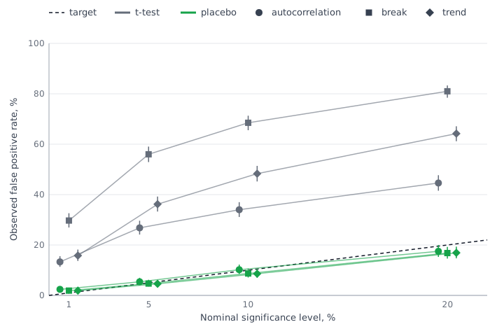
Closed-form intervals are for learning. The t-based interval above assumes independent residuals. Real daily and weekly KPI series are autocorrelated and drift, and in A/A simulations built on data from 192 advertisers, the GeoX paper found that plain t-tests at a 5% nominal level produced more than ten times the expected false positives. GeoX therefore uses design-aware placebo inference and GeoLift uses conformal inference by default. For a budget decision, use the library's inference, not a spreadsheet t-test.
Other estimators: GBR, Trimmed Match, synthetic control and ASCM
Geo-based regression (GBR)
Vaver and Koehler's 2011 method is the original Google approach.² It collapses time instead of regions: one row per region, with totals for the pre-period and the test period.
and are the KPI totals of region g in the pre-period and the test period, is its incremental spend (zero in control regions), is the iROAS, and the regression is weighted by to handle regions of different size. GBR draws its statistical power from the number of regions, which is exactly why Kerman et al. developed TBR for markets with few of them.⁷ With about 20 regions, GBR is not my first choice.
Trimmed Match
Chen and Au (Annals of Applied Statistics, 2022) built Trimmed Match for randomised paired geo experiments with few, highly heterogeneous regions.⁸ For each pair i, take the treatment-minus-control differences in response, , and in spend, , over the test period. For a candidate iROAS r the pair's residual is
and the estimate is the r at which the trimmed mean of these residuals is zero, which works out to
where is the set of trimmed pairs, those with the most extreme residuals. A single badly matched pair, say a city with a one-off event, cannot drive the answer, and the trim level is chosen from the data. The estimator is distribution-free; Google's open-source trimmed_match library implements it. The limit for small markets is arithmetic: 20 regions make at most 10 pairs, and trimming spends some of them.
Synthetic control and ASCM (GeoLift)
A synthetic control builds the counterfactual as a weighted average of individual control regions rather than their plain sum:³
Region 1 is the treated unit, C is the set of control regions, and the weights are chosen so that the weighted controls reproduce the treated unit's pre-period path. The constraint keeps the forecast inside the range of the controls, which is safe but fails when no mix of controls fits the pre-period well; the original authors advise against using synthetic control in that case.⁹ The augmented synthetic control method (ASCM) of Ben-Michael, Feller and Rothstein estimates the bias left by the imperfect fit with an outcome model and subtracts it:⁹
is the outcome model's prediction (ridge regression in the authors' main proposal), so the first term is the plain synthetic control and the bracket is the estimated bias from imperfect pre-period fit. If the fit is already good, the correction is small; if not, ASCM extrapolates a little beyond the controls, and the ridge penalty limits how far.⁹
GeoLift, Meta's open-source R package, uses ASCM to estimate and de-bias the synthetic control.⁵ It adds power calculators and market selection, and reports the average treatment effect on the treated, percent lift, incremental KPI, a confidence interval and a p-value. It has no native iROAS output: divide the incremental revenue by the test spend yourself. As of October 2026 the GitHub main branch carries version 2.7.5, the last tagged release is v2.6.06 from May 2023, and the package is installed from GitHub rather than CRAN.⁵
GeoX, as of October 2026, is the meridian-geox Python package (1.0.0 released 1 September 2026, Apache-2.0).⁴ Its white paper describes TBR, synthetic control and synthetic difference-in-differences and argues that the unit-weighting methods do better when the region pool contains outsized regions or very noisy series;³ in the open-source code, only TBR runs today.⁴ Google's paper also benchmarks GeoX against an unnamed open-source ASCM library and reports the same median minimum detectable effect (6%) with lower required budgets; that is the vendor's own evaluation, so read it as such.³
Which method when
| Situation | Method | Tool |
|---|---|---|
| Dozens of regions or more, randomised or stratified assignment | TBR (GBR also works) | GeoX |
| Randomised pairs, a few pairs likely to be badly matched | Trimmed Match | trimmed_match |
| Few regions, or one or two outsized regions that cannot be randomised | Synthetic control with ASCM, matched markets | GeoLift |
| One test region against one control region | TBR runs on two regions, without randomisation's protection | GeoX, GeoLift |
| National-only channel that cannot be split by region | Not a geo test: a before-and-after study with a synthetic control, or a wide MMM prior | CausalImpact, MMM |
The last row comes from Google's playbook, which suggests a Causal Impact study when a channel such as TV or OOH cannot be bought by region, noting that it still needs a period with and a period without advertising.¹
Uncertainty: placebo inference instead of a t-test
The interval is where most geo tests go wrong. A t-test that compares the test regions with their own history assumes independent days, but daily sales are autocorrelated, and a shock that hits every region at once (a holiday, a price change, a competitor's launch) looks exactly like a treatment effect. Google's Meridian GeoX paper replaces the parametric test with placebo inference: pretend that some control regions were treated, measure the effect found there, repeat many times, and use that distribution as the null.³
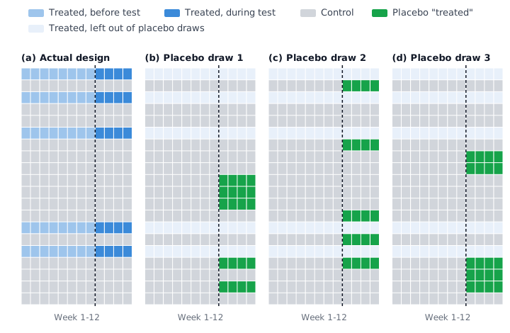
The simulation below follows the paper's A/A evaluation on a panel shaped like Kazakhstan: 20 regions, 56 days before the test and 28 during it, 5 regions treated at random and no real effect anywhere. Each scenario runs 1,000 A/A tests. A valid method gives a flat histogram of p-values and flags about 5% of tests at the 5% level.
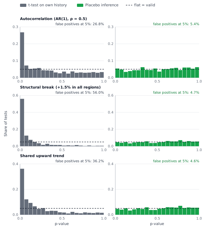
With autocorrelated noise (AR(1), ρ = 0.5) the t-test flags 26.8% of the tests; with a +1.5% shift that hits all regions a week into the test, 56.0%; with a shared upward trend, 36.2%. Placebo inference stays at 5.4%, 4.7% and 4.6%, because it compares the test regions with regions that went through the same shock at the same time.
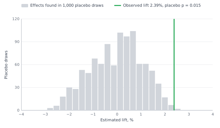
With a real effect the same machinery gives the p-value and the interval. In a simulated test with a true 3% lift in five regions the estimate is 2.39%. Only 14 of 1,000 placebo draws produce an effect at least that large, so p = 0.015; the spread of the placebo effects, 1.09 percentage points, gives an approximate 90% interval of 0.59% to 4.18%.
Power, minimum detectable effect and test length
A geo test is a bet that the effect is big enough to see through the noise of regional sales. GeoLift's methodology page makes the point directly: without a power analysis before the test, there is a high chance of failing to find a lift that actually happened.⁵ The power analysis gives you the minimum detectable effect (MDE): the smallest effect the design would detect with the chosen confidence and power.
- 3x: pre-period vs test length, GeoX minimum
- 4-5x: pre-period vs test length, GeoLift recommendation
- 25 and 20+: pre-treatment periods and geo units, GeoLift minimum
- 7-14 weeks: GeoX timeline from planning to finished analysis
GeoX defines the MDE as:³
is the standard error of the incremental response, Baseline is the treatment group's response without the intervention, α is the significance level and π the target power; GeoX's defaults are a two-sided α = 0.1 (90% confidence) and π = 0.8, which give z-values of 1.645 and 0.842.⁴ For a new activation the budget needed to reach that MDE follows directly:³
Apply this to the worked example. With a standard error of $5.24k, the detectable effect is , i.e. $13.0k, or 1.4% of the $956.1k baseline. The heavy-up produced $33.2k, comfortably above it. Now suppose the same test had added only $5k of spend: at the same iROAS of 1.66 the expected effect is about $8.3k (5 × 1.66), below the $13.0k MDE, and the test would most likely have come back "not significant" whatever the truth. By the budget formula, at iROAS 1.66 (a cost of 1 / 1.66 = 0.60 per incremental dollar) the minimum extra spend for this design is about 13.0 × 0.60 = $7.8k. In a real design you estimate the standard error before the test, from history: Kerman et al. slide a window of the planned test length through past data, compute the interval for each pseudo-experiment and take the median,⁷ and GeoX and GeoLift run the equivalent simulations for you.
For a sense of scale: across the 69 advertiser studies in the GeoX paper's benchmark, the median MDE of the selected designs was 6%.³ A channel you expect to move sales by 2% is not testable with a typical design, however much you want the answer.
A test that cannot detect the expected effect is wasted money. If the power analysis says the MDE is above the effect you realistically expect, the test will most likely end "not significant" regardless of the truth. You will have paid for the media, the sales lost in go-dark regions and the analyst time, and learned nothing a prior could not have told you. Change the design (more spend, longer test, more regions, a less noisy KPI) or do not run it.
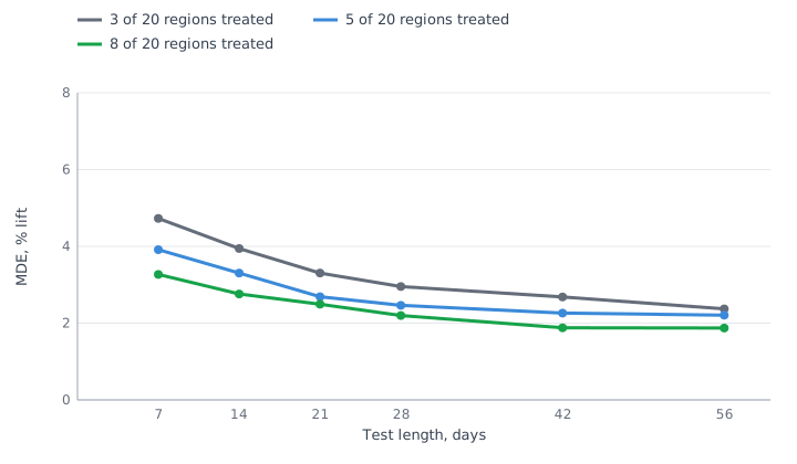
On the same simulated panel, with 5 of 20 regions treated, the minimum detectable lift falls from 3.91% for a one-week test to 2.46% at four weeks and 2.21% at eight. At four weeks, treating 8 regions instead of 3 lowers it from 2.95% to 2.20%, more than doubling a three-region test to eight weeks does (2.37%). These values depend on the simulated noise, 5% a day with ρ = 0.5; your own come from the same calculation on your own history.
What moves the MDE
Kerman et al. list the levers in order of strength:⁷
- Spend intensity. The most influential parameter: doubling the spend change per week halves the width of the iROAS interval. The catch is that more spend also pushes further into diminishing returns.
- Pre-period length. The interval half-width falls roughly with the square root of the number of pre-period points, with a floor it cannot go below.
- Test length. Longer helps as long as spend intensity holds, with diminishing gains.
- Regions. The number of regions does not enter TBR directly, but very few regions mean a worse fit and a noisier counterfactual. A high correlation between treatment and control series improves the fit.
Duration guidance from the two libraries:
- GeoX: planning up to 2 weeks, an active test of 3 to 10 weeks, and a cool-down of 2 weeks or more when conversions lag, 7 to 14 weeks in total; at least 3x the test length in pre-period data, split into training, validation and evaluation, and more when the KPI is seasonal.¹⁰ ³
- GeoLift: daily data strongly preferred over weekly; a pre-period of 4 to 5 times the test length with no structural breaks; at least 25 pre-treatment periods and 20 or more geo units; about 52 weeks of history to cover seasonality; a test of at least 15 days with daily data or 4 to 6 weeks with weekly data, covering at least one purchase cycle.¹¹
Long sales cycles need extra care. A loan application that turns into a disbursement three weeks later, or a mortgage that closes in two months, may land after the test ends. Google's playbook suggests measuring a micro-conversion that predicts the sale (an application, an approval) when the cycle is longer than the test, and choosing it by correlation analysis.¹ If you go that way, check that the micro-conversion is what the money follows; the Google Ads leads without disbursements article shows how far the two can drift apart.
Kazakhstan and the CIS: twenty regions and two giants
Kazakhstan has 17 oblasts and 3 cities of republican significance (Almaty, Astana and Shymkent): about 20 geo units. Google's geo-testing papers start from the 210 Nielsen DMAs of the US.⁷ For most businesses Almaty and Astana carry a disproportionate share of volume. That puts a Kazakhstan test at or just below GeoLift's minimum of 20 geo units, far from the comfort of randomising 210, and squarely in the situation the GeoX paper names as a main cost driver: disproportionately large regions, such as New York or London in their examples, that have no comparable match.³ The same logic applies to any market with a few dozen first-level regions or fewer.
What I would do about it:
- Assignment. Fix the role of the giants. Do not let a random draw put Almaty or Astana into treatment. Either keep both out of the experiment (business as usual, excluded from the analysis) and test on the remaining regions, or, if a big city must be tested, use a synthetic control in GeoLift with all other regions as donors. TBR's plain aggregation handles outsized regions worst.
- Granularity. Split regions where the KPI allows. Oblast centres and the rest of the oblast, or large cities as their own units, can roughly double the count, but only if every platform in the test can target them separately and your backend assigns each order or application to the unit reliably. Kerman et al. built 29 geos for France from targetable cities. Do not go too small: Vaver and Koehler warn that units as small as postal codes are not workable, because ad serving is imprecise and people cross boundaries.
- Design. Stratify or pair. With 20 units, a pure coin flip is a gamble. Use stratified assignment (the GeoX default) or pair regions by size and randomise within pairs, and check the A/A result on the pre-period before launch.
- Intervention. Go dark on smaller regions. Switching a channel off in a group of smaller oblasts caps the revenue at risk, and a go-dark is measured against zero spend, which is what MMM priors need. The spend you remove must still be large relative to those regions' noise: run the power analysis on exactly those regions.
- Time. Run longer, accept a bigger MDE. With few units, time is the lever left: a longer pre-period, a test toward the 10-week end of the GeoX range, daily data where the KPI allows. Agree in advance what MDE the business can live with; if it is above the plausible effect, stop.
- Fallback. Know when it is not testable. If no design brings the MDE under the plausible effect, use a national on-off period read with a Causal Impact study, or keep the channel's MMM prior wide and say so in the report. A wide prior is honest; a fake experiment is not.
Data prerequisites
Most geo tests I see stall on data, not statistics. Before any design work:
- KPI by region by day from the backend. Orders, loan applications, approved loans, issued policies, deposits: whatever the business counts as the outcome, summable across regions and days. Not platform-reported conversions: GeoX's implementation guide asks for raw, unfiltered conversion events rather than attributed ones.¹⁰ If the KPI lives in several systems, the first-party data warehouse article covers how to bring it together.
- One stable geo key per record. Decide which region an order belongs to: delivery address, servicing branch, customer's registration, or IP-based city. Pick one, keep it as close as possible to how the ads are targeted, and do not mix definitions. Offline conversions from branches and call centres need the region from the CRM.
- Spend by region by day for every platform in the test. Most ad platforms offer a location breakdown in reporting; check before the test that the export works at your region level and reconciles with billing.
- Clean history. At least 52 weeks with a value for every region and date (GeoLift does not accept gaps), ideally two years so seasonality is visible.¹¹
- A log of everything regional. Local promotions, branch openings, outages, regional TV. GeoLift's best practices ask for local marketing to be held constant across test and control regions.¹¹
Feeding the result into MMM
An experiment measures one channel, in one period, at one spend level. An MMM needs that channel's whole response curve over years. So the experiment informs the model; it does not replace it. Google's playbook gives the working rules:¹
- Validate before you calibrate. Compare the MMM's ROI with the experiment's iROAS for the same channel, KPI and period. A difference of 5 to 10% is acceptable and needs no action; above 10%, calibrate the model with the experiment.
- Do not calibrate a full channel from a single experiment. The playbook lists this as a pitfall and treats calibration as continuous. It also notes that one experiment can be a good source for a prior when the channel is run the same way over time and seasonality is weak: one test can shape a prior, it should not dictate the answer.
- Never use the same experiment to validate and to calibrate the same model. Once a result has gone into a prior, the next validation needs a new test.
- Move budget in steps. When acting on MMM forecasts, shift at most 20% of a channel's spend at a time, and validate changes above 10% with an experiment where feasible.
- Test where the model is least sure. Channels with the widest ROI intervals get the next experiment.
How each library takes the result:
| Library | How the experiment enters | What it uses | Watch out |
|---|---|---|---|
| Meridian 2.0+ | ROI prior for the tested channel, built by CalibrationBuilder | iCPD point estimate and standard deviation, business-as-usual spend, dates | Built for a zero-spend counterfactual: holdback and go-dark fit, heavy-up does not directly |
| Robyn | A calibration_input row; MAPE.LIFT becomes a third objective | Point estimate only | The interval is ignored; the test must sit inside the modelling window |
| PyMC-Marketing | add_lift_test_measurements adds a likelihood term | Spend level, spend change, lift and its standard deviation | A natural fit for heavy-ups |
Meridian
Meridian puts its priors on ROI rather than on raw coefficients, so an experiment translates into a prior directly. Since version 2.0 (September 2026), CalibrationBuilder accepts a GeoX analysis result and reads the iCPD point estimate and standard deviation, the estimated business-as-usual spend and the analysis dates.¹² ¹³ It then adjusts for three mismatches between the test and the model: spend level (experiment vs channel average daily spend), recency (a 52-week half-life, so older tests count less) and duration (a short test captures only part of the adstock carryover), merges several experiments by Bayesian updating and fits a parametric prior.¹³ The documentation is explicit that the builder is designed for lift experiments measured against a zero-spend baseline and warns that a non-zero counterfactual creates an estimand mismatch.¹³ A heavy-up has a non-zero counterfactual, business-as-usual spend, so by that logic it does not fit directly: our heavy-up's 1.66 is closer to a marginal return than to the channel's average ROI. As of October 2026 the Meridian changelog also lists an unreleased fix to make calibrated ROI priors on the JAX backend match TensorFlow, so check the release notes before relying on calibrated priors on the default backend.¹² The Meridian article covers the rest of the setup.
Robyn
Robyn takes experiments as rows of calibration_input (channel, liftStartDate, liftEndDate, liftAbs, spend, confidence, metric, calibration_scope) and adds a third objective to its search:¹⁴
is the lift measured by experiment k (liftAbs), is the model's decomposed contribution of that channel over the same window, and K is the number of experiments. By default only models in the best 10% on MAPE.LIFT go forward to the usual Pareto selection.¹⁴ Robyn's analyst guide states that it accepts only a point estimate as calibration input,¹⁵ so $33.2k enters as if it were exact and the $23.0k to $43.4k interval is lost. In my reading, is the channel's contribution against zero spend, so holdback and go-dark results compare naturally, while a heavy-up's lift covers only the extra spend and should not be passed as the whole channel's lift.
PyMC-Marketing
PyMC-Marketing's add_lift_test_measurements takes the channel, the spend level x, the spend change Δx, the measured lift Δy and its standard deviation σ. The documentation describes a lift test as two points on the channel's saturation curve, and the method adds a likelihood term:¹⁶
Here f is the channel's saturation curve including its coefficient β, and it lives on the model's own grain: one period (a week in a weekly model) and, in a regional model, one region. The method compares two points on that curve; it does not add up predictions over the weeks of the experiment. So the test result has to be converted before it goes in, not passed as window totals. For the heavy-up in this article that means weekly values: Δx = 20 / 4 = 5, Δy = 33.2 / 4 = 8.3 and σ = 5.24 / 4 ≈ 1.31 ($k per week), with x the weekly business-as-usual spend of the channel in the treatment regions. In a regional model, pass one row per test region and split the lift between them, for example in proportion to each region's baseline; in a national model, x and Δx have to be on the same scale as the national spend the model sees, because the test covered only part of the country.
The weekly conversion rests on two assumptions worth checking. First, spend was held steady through the test. Second, the test was long compared with the channel's carryover, so the adstocked spend had time to settle at its new level: with normalised adstock, which PyMC-Marketing uses by default, a steady weekly spend x has an adstocked value of x. Carryover that arrives after the test window is not in Δy at all, so for slow-decaying channels the conversion understates the effect; a longer test or a cool-down inside the measured window does more for those than any arithmetic. A holdback or a go-dark is the same construction with the pair of points 0 and the weekly test spend. For those two designs there is also a window-level alternative: add_cost_per_target_calibration puts a likelihood on the channel's ROAS or cost per result over a date range, so the test's iROAS can be used for the test dates directly. So when heavy-ups are your main design, PyMC-Marketing is the most direct consumer, as long as the conversion above holds; the library comparison goes into the rest of the trade-offs.
The loop
The experiment and the model feed each other: the model points at the channel it is least sure about, the experiment narrows it, and the next refresh points somewhere else.
A geo test, from question to MMM
No test unless the MDE is below the expected effect
Question
Widest ROI interval in the MMM
Hypothesis and KPI
Design
Power analysis and MDE
Assign regions
- freeze other changes
Run
Test period
Cool-down
Read and use
Lift with its interval
Budget decision
Prior or lift term in the MMM
- placebo inference
The calibrated MMM points to the next channel to test.
Meridian 2.0 helps with the first box: its channel calibration recommendations score channels on implausibly high or low ROI, wide posteriors and a potential-bias check against control variables, and flag the ones that would gain most from an experiment.¹⁷
Run checklist
- Hypothesis written with the decision attached: if iROAS clears the threshold, we do X; if not, we do Y
- KPI defined and pulled from the backend by region and day, with the same definition the MMM uses
- Geo units defined, targetable on every platform in the test, KPI tagged to them reliably
- Clean pre-period of at least 3x (GeoX) to 4-5x (GeoLift) the test length; 52 weeks for seasonality
- Power analysis done: MDE and required budget known, expected effect above the MDE
- Design chosen to match the question and how the result will enter the MMM: holdback, go-dark or heavy-up
- Assignment by stratified or paired randomisation, role of the largest cities fixed in advance, A/A check passed
- Targeting locked: physical presence only, regions targeted positively, no concurrent lift studies on the same campaigns
- Freeze list agreed: no region swaps, no budget moves between regions, local promotions balanced or logged
- Test run for the planned length plus cool-down, no early stopping
- Result read with interval and p-value, design quality (fit, A/A, MDE) checked before trusting it
- Decision taken against the pre-agreed threshold
- Result fed to the MMM as a prior or lift term, or kept aside for validation, and the choice logged
Mistakes that make a geo test worthless
Peeking and stopping early
Checking the result every few days and stopping the first time it looks significant inflates the false-positive rate far above the nominal 10%. Early cumulative iROAS is unstable by nature, as Kerman et al. show. Fix the end date in the plan and read the result once, at the end of the cool-down.
Contaminated regions and spillover
People who live in a control region and work in a treatment one, delivery addresses that differ from where the ad was seen, location targeting by "presence or interest", a national campaign that leaks into everything, a brand lift study running on the same campaigns. GeoX's guide asks for physical-presence targeting, positive targeting of each region and no concurrent lift or holdout studies. Spillover usually pulls the measured effect toward zero.
A pre-period that is too short
The worked example uses 8 pre-period weeks for a 4-week test, 2x, and its point estimate misses the true effect by 13%. GeoX asks for at least 3x the test length and GeoLift for 4-5x and at least 25 periods. A pre-period with a structural break (a repricing, a new branch network, a tracking change) is worse than a short clean one.
Platform conversions as the KPI
Attributed or platform-modelled conversions count only what the platform sees and credits, so the test ends up measuring the platform's attribution, not your business. Consent rules and browser restrictions shrink that view further, as the Consent Mode v2 article explains. Use raw backend events: orders, applications, policies.
Changing budgets or regions mid-test
Moving budget from treatment to control regions, adding a region because it underperforms, launching a promotion in treatment regions only: each one breaks the counterfactual. GeoX's guide forbids adding, removing or swapping regions during the test, and GeoLift asks for all other media to be held constant across markets.
Next step
The practical next step: pull 52 weeks of your main KPI by region and day from the backend and run a GeoX or GeoLift power analysis on it. That alone tells you which channels can be tested at all.
Sources
¹ Modern Measurement playbook: MEM guidelines and best practices - Google
² Measuring Ad Effectiveness Using Geo Experiments (Vaver, Koehler, 2011) - Google Research
³ Meridian GeoX: An Open-Source Framework for Precision and Efficiency in Geo Experiments (Ye, Sinn, Li, Jiao, 2026) - Google Research
⁴ google/meridian-geox - GitHub
⁵ facebookincubator/GeoLift - GitHub
⁶ Types of experiments - Meridian GeoX, Google for Developers
⁷ Estimating Ad Effectiveness using Geo Experiments in a Time-Based Regression Framework (Kerman, Wang, Vaver, 2017) - Google Research
⁸ Robust Causal Inference for Incremental Return on Ad Spend with Randomized Paired Geo Experiments (Chen, Au) - Annals of Applied Statistics 16(1), 2022; arXiv
⁹ The Augmented Synthetic Control Method (Ben-Michael, Feller, Rothstein) - Journal of the American Statistical Association 116(536), 2021
¹⁰ Implementation of geo testing - Meridian GeoX, Google for Developers
¹¹ GeoLift Best Practices - Meta Open Source
¹² Meridian CHANGELOG - GitHub
¹³ Set custom ROI priors using past experiments - Meridian, Google for Developers
¹⁴ Robyn features: calibration - Meta Open Source
¹⁵ Analyst's guide to MMM - Robyn, Meta Open Source
¹⁶ Lift test calibration - PyMC-Marketing documentation
¹⁷ Channel calibration recommendation and score - Meridian, Google for Developers
FAQ
Can we run a geo test with just two cities, say Almaty as treatment and Astana as control?
Technically yes: TBR works with one test and one control region, which is how matched-market tests run. But nothing protects you from whatever happens in one city and not the other during the test, such as a competitor's promotion, a local holiday or an outage, and it all lands in your estimate. If you must, use a long clean pre-period, check the pre-period fit, prefer a synthetic control built from several regions over a single control city, and treat the result as directional.
The result came back not significant. Does that mean the channel does not work?
No. It means the test did not give enough evidence against zero at the threshold you chose; it does not show that the effect is zero or even that it is small, because a real effect at the MDE is still missed about one time in five at 80% power. Read the confidence interval instead: it lists the effect sizes that remain compatible with the data. If it spans both unprofitable and very profitable values, the test was underpowered for your decision. You can still pass the estimate with its wide standard deviation to Meridian as a weak prior, but do not pass it to Robyn, which would treat the point estimate as exact.
How often should we repeat a geo test on the same channel?
Effects drift with creative, competition and saturation, so a test result ages. Meridian's calibration discounts older experiments with a 52-week half-life, and Google's playbook suggests a learning agenda with a geo experiment once a year, complemented by lighter conversion lift studies in between. In practice I retest a major channel about yearly and after any large change in its spend level or strategy.
Can we geo-test TV or outdoor advertising?
Outdoor usually yes: it is bought by city, so a holdback or go-dark by city works if your KPI is tagged to the same cities. National TV cannot be split by region, so it cannot be a geo test; Google's playbook suggests a Causal Impact study on a period with and without advertising, or relying on the MMM with an honest, wide prior. Regional TV, where it can be bought separately, is tested like any other regional channel.
Do we need GeoX or GeoLift, or can an analyst do this in a spreadsheet?
The TBR point estimate is a regression you can run in a spreadsheet, as the worked example shows. The hard parts are design and inference: stratified assignment with A/A checks, simulated power and MDE, and intervals that hold up when the KPI series is autocorrelated, where the GeoX paper found plain t-tests gave more than ten times the expected false positives. That is what the libraries give you, so use one for any test that will move budget.
Seeing this in your own funnel?
Two weeks, fixed scope, read-only access. You get the findings and a 90-day roadmap whether or not we work together afterwards.