
Meridian is Google's open-source Bayesian marketing mix model, at version 2.1.0 as of October 2026. It pays back its setup cost when you have at least two years of weekly data split by region (three years if you only have national totals), several channels whose spend actually moved over time, and someone who reads the diagnostics before the charts. Its headline number, ROI, tells you how a channel did on average. The budget decision needs marginal ROI, and in the worked example below a channel with an ROI of 2.0 returns only 0.667 on the next dollar.
Where Meridian stands in October 2026
Meridian is a Python library that fits a geo-level Bayesian hierarchical media mix model.¹ Google opened it to all advertisers in January 2025² and it replaced LightweightMMM, whose repository is now archived with a note that it is no longer supported.³
The state of the release line as of October 2026:
-
Version. The latest release is 2.1.0: changelog dated 17 September 2026, on PyPI since 25 September 2026. Version 2.0.0 was dated 2 September 2026.⁴ ⁵
-
What 2.0 changed. The default computation backend switched from TensorFlow to JAX, and the library gained prior calibration through incrementality experiments such as Meridian GeoX, plus channel calibration recommendations.⁴
-
What 2.1 changed. A declarative vocabulary in
ModelSpec: calibration windows and holdouts are now named by channel, geo and date (DateRange,CalibrationSpec,HoldoutSpec) instead of raw index arrays.⁴ -
License and runtime. Apache-2.0. The README requires Python 3.11 to 3.13 and recommends at least one GPU; it states the project was tested on a T4 GPU with 16 GB of RAM.⁶
-
Estimation. Parameters are sampled with the No-U-Turn Sampler (NUTS), a Markov chain Monte Carlo (MCMC) method that is compute-heavy, which is why the GPU recommendation exists.⁶
-
2.1.0: latest release, September 2026
-
2 years: weekly geo-level data, minimum
-
3 years: for a national-only model
-
1 GPU: recommended minimum for fitting
The model is an extension of two Google papers: Jin et al. (2017), which put adstock and Hill saturation into a Bayesian MMM,⁷ and Sun et al. (2017), which added the geo-level hierarchy.⁸ Meridian adds reach and frequency inputs, a time-varying intercept for trend and seasonality, organic media and non-media treatments.¹ Around the library Google now ships Meridian GeoX for geo experiments and a Scenario Planner, a notebook-generated report with interactive budget scenarios that the docs still label as beta.⁹
If MMM itself is new to you, start with the series hub, Marketing mix modeling: what it measures, how it works and when it pays off. The question here is narrower: is Meridian the right tool, and once it runs, how do you read it?
- Good fit. Several channels, regional data. Several paid channels, at least two years of weekly KPI and spend by region, and spend that changed over time. An analyst who can run Python and read posterior diagnostics.
- Good fit. You run or plan experiments. Meridian puts its priors on ROI, so every geo test or lift study can feed the model directly. If you test, Meridian turns tests into a measurement system rather than one-off reports.
- Poor fit. Short or flat history. Less than two years of data, or channels that ran at the same level every week. The model then has to extrapolate the zero-spend scenario from its assumptions, and the posterior mostly repeats the prior.
- Poor fit. Campaign-level questions. Meridian works at channel level and Google advises against campaign-level models. Creative and campaign decisions belong to platform experiments and attribution.
If your team works in R, or you want a different modelling philosophy, the comparison in Meridian vs Robyn vs PyMC-Marketing covers the trade-offs.
The model in Meridian's notation
Meridian's full specification has blocks for paid media, organic media, non-media treatments and reach-and-frequency channels.¹ The core that matters for most advertisers is this:
Here y is the KPI in geo g and week t, μ is a time effect shared by all geos, τ is a geo intercept, z is control variable i with geo-level coefficient γ, x is paid media of channel i, β is that channel's geo-level effect, L is the maximum lag, α, ec and slope are the channel's decay, half-saturation and shape parameters, and ε is the error.
Two notes before the pieces. First, notation: in the series hub I used θ for geometric decay and s for the Hill slope; Meridian calls them α and slope and uses s as the lag index, so I follow Meridian here. Second, scaling: the KPI is divided by geo population and then centred to mean zero and scaled to standard deviation one, and media is scaled per capita and by the channel's median, so the parameters live on a standardised scale rather than in dollars.¹⁰
Baseline: geo intercepts and time effects
One geo is the reference with τ = 0 (by default the one with the largest population); every other geo gets its own intercept with a Normal(0, 5) prior.¹¹ The time effect μ is a weighted average of the two nearest knot values:
Here b are the knot values, ℓ(t) and u(t) are the nearest knots before and after week t, and w(t) is a linear weight that favours the closer knot.¹ By default a geo model gets one knot per week, which it can afford because every week is observed in many geos; a national model gets a single knot, which is one common intercept with no trend unless you add knots. The baseline moves over time, but media effectiveness does not: Meridian does not model it as time-varying.¹²
Adstock: carryover, normalised
Here x is media in week t minus s, w is the weight of lag s, α between 0 and 1 is the decay rate and L is the maximum lag (max_lag, default 8 weeks). Geometric decay is the default; the alternative binomial weight suits channels whose effect persists into the second half of the window. The docs suggest max_lag of 2 to 10 weeks for geometric and 4 to 20 for binomial decay, and the default α prior is Uniform(0, 1).¹³
The detail people miss is the denominator. In the series hub a single burst of 100 with a decay of 0.6 accumulates to about 250 over time, because raw geometric weights sum to 1/(1 − 0.6). Meridian divides by the sum of the weights, so the same burst is spread over the following weeks but its total stays 100; the size of the effect lives entirely in β. A useful consequence: if a channel runs at a constant weekly level x, its adstocked value is exactly x, which keeps the worked example below exact in steady state.
Hill: saturation
Here ec is the media level at which the effect reaches half of its maximum, and slope sets the shape: at or below 1 the curve is concave from the start, above 1 it is S-shaped.¹⁴ By default Meridian applies Hill to the adstocked media, and for ordinary (non reach-and-frequency) channels it fixes slope at 1 with a Deterministic(1) prior. The docs give the reason: the budget optimiser finds a global optimum only when curves are concave, and S-shaped curves can cause convergence problems.¹¹ The ec prior is TruncatedNormal(0.8, 0.8, 0.1, 10) on the scaled axis, where ec = 1 means half-saturation at the channel's median non-zero media per capita.¹¹
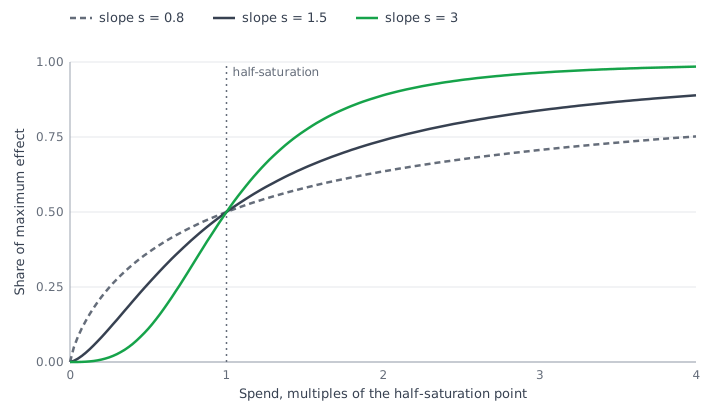
The docs add a warning worth repeating: the Hill parameters are estimated from the spend range you actually observed, and curve points outside that range are extrapolation.¹⁴
Hierarchy across geos
Each geo g gets its own effect for channel i, drawn around the channel-level mean β with spread η. This is the default log-normal form; a normal form is available.¹ The η prior is HalfNormal(1), which the docs describe as moderate regularisation that encourages pooling across geos.¹¹ Controls get the same treatment, with γ for geo g drawn from Normal(γ, ξ) and a weaker pooling prior on ξ. Decay, ec and slope are shared by all geos within a channel. In plain words: every region has its own media effect, pulled towards the channel average, and small regions borrow strength from large ones. That is the Sun et al. idea, and it is why geo data gives tighter intervals than national data.⁸
Likelihood
The residual for geo g and week t is normal with standard deviation σ. By default all geos share one σ (unique_sigma_for_each_geo=False), which means small, noisy geos can sway the fit; the docs advise dropping the smallest geos by KPI first.¹⁵
The Bayesian step in one paragraph
Θ stands for all model parameters, p(Θ) is the prior (what you believe before seeing the data), p(y | Θ) is the likelihood defined by the model above, and p(Θ | y) is the posterior.¹⁶ Meridian draws samples from the posterior with NUTS; the docs' example runs 7 chains with 1,000 adaptation draws, 500 burn-in draws and 1,000 kept draws per chain.¹⁷ Every output, from ROI to response curves, is computed draw by draw, so you get a distribution rather than a number, and the default summaries are 90% credible intervals. When the data carries little information about a channel, the posterior stays close to the prior. That single fact is why the next section matters more than any other setting.
Reach and frequency channels
For channels with reach r and average frequency f per geo-week, Meridian replaces impressions with this term:¹⁸
Reach enters linearly, frequency goes through Hill, and here the slope is learned, so the frequency curve may be S-shaped. The default priors on ec and slope for these channels are set so that the prior optimal frequency has a mean of 2.1 and a 90% interval of 1.0 to 4.4.¹¹ Reach must be unique people per period (not cumulative) and frequency is impressions divided by reach, at the same geo-week grain as the KPI.¹⁸ The output is an optimal frequency per channel, the frequency that maximises ROI, applied equally across geos and weeks; the budget optimiser uses it by default.¹⁹ The docs point to Google's MMM Data Platform for YouTube reach and frequency; for other channels you need your own data at that grain.
Priors on ROI: the setting that matters most
The coefficient β has no business meaning. The same β implies very different ROIs for two channels, because ROI also depends on cost per media unit, flighting, adstock and saturation. Meridian therefore re-parameterises the model so that the prior sits on ROI and β is derived from it:²⁰
Here M is the channel's transformed media expressed in outcome units per unit of β (it carries the population and KPI scaling), and x with a tilde is the channel's spend in geo g and week t. Once decay, half-saturation and the geo deviations are fixed, β and ROI map one to one, so Meridian can sample ROI from its prior and compute β.²⁰
The default prior for every paid channel is LogNormal(0.2, 0.9). In the docs' words it puts the mean ROI at 1.83, half of the mass above 1.22, 80% between 0.5 and 6.0 and 95% between 0.25 and 9.0.¹¹ Those two ranges do not match the distribution itself: the quantiles of LogNormal(0.2, 0.9) are about 0.39 to 3.9 for 80% and 0.21 to 7.1 for 95% ( and ), while the mean of 1.83 and the median of 1.22 are right. Plot the prior before you reason about it. It is the same for every channel, so a priori no channel is favoured on ROI.
Why this matters for calibration: an experiment measures incremental outcome per unit of spend, which is an ROI. With ROI priors, an experiment result can be written straight into the prior. With priors on β, it could not.
Three other prior types exist for paid media.²¹
| Prior type | What you state | Default | When to use |
|---|---|---|---|
| ROI (default) | Incremental outcome per unit of spend | LogNormal(0.2, 0.9) | Almost always; this is where experiments plug in |
| mROI | Return on a small spend increase | LogNormal(0.0, 0.5) | A common mROI prior shrinks recommended budget shifts towards the historical mix |
| Contribution | Share of total outcome | Beta(1, 99), mean 1% | Organic media and non-media treatments (the default there) |
| Coefficient | β directly | HalfNormal(5) | Rarely; Google itself rarely recommends it |
If the KPI is not revenue and you provide no revenue per KPI, the ROI prior is replaced by a prior on the total contribution of paid media, with a mean of 40% and a standard deviation of 20%.¹¹ The docs frame a calibrated prior as a guardrail: weak or no guardrails are tempting, but without a reasonable prior the model can decide that a low-spend channel drives massive revenue.²²
What the prior and one experiment do to a channel
The two figures use the simulated brand from the MMM overview: two years of weekly data, three channels with known true ROI (search 2.5, video 1.8, outdoor 1.2) and Meridian's default ROI prior, LogNormal(0.2, 0.9), whose 90% interval runs from 0.28 to 4.69. The posteriors are computed on a grid with a normal approximation to the data likelihood, which keeps the picture exact and reproducible; Meridian itself samples the full model with NUTS.
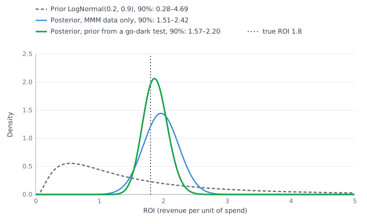
Video always runs in the same high-season weeks, so the data cannot fully separate it from seasonality: on their own they put its ROI at 1.96, with a 90% interval of 1.51 to 2.42. Calibration replaces the default prior with one built from an experiment whose counterfactual is zero spend. Here that is a simulated go-dark test that switches video off for four weeks in part of the country, withholds $60k of spend and measures an ROI of 1.77 with a standard error of 0.25, which gives a log-normal prior with a 90% interval of 1.39 to 2.21. With it the posterior narrows to 1.57 to 2.20 and its mean moves from 1.96 to 1.88, closer to the true 1.8. A heavy-up such as the worked example in the geo experiments article would be the wrong input here: it measures the return on extra spend, not the average ROI that the prior describes.
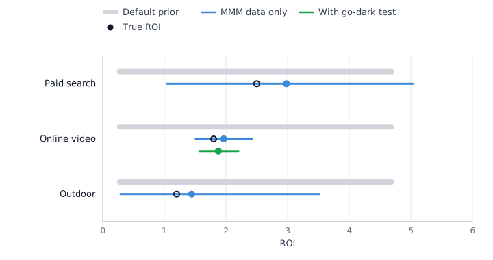
Ask for this view in every report. Search spend moves with the season too, and its interval stays wide, 1.04 to 5.03. Outdoor spend barely changes from week to week, so the data say little: its interval of 0.29 to 3.52 is close to the prior's 0.28 to 4.69, which means the outdoor ROI in such a report is mostly the prior you chose.
What data Meridian needs
| Item | Meridian guidance |
|---|---|
| Granularity | Weekly is the best practice; daily or monthly are acceptable alternatives, but daily data lengthens runtime and monthly data can give wide intervals or fail to converge |
| History, geo model | At least two years of weekly data |
| History, national model | At least three years |
| Monthly data only | At least three years |
| KPI | Must add up across geos and weeks (sales, accounts, conversions); ROI in money needs revenue or revenue per KPI |
| Population | Required per geo, used to scale KPI and media |
| National-only media | Impute to geos by population share and still run a geo model |
| Level of detail | Channel level; campaign-level models are not recommended |
Sources for the table: the data collection,²³ geo selection¹⁵ and data sufficiency²⁴ pages.
The data-sufficiency page gives two worked examples that are worth knowing by heart.²⁴
- 4: data points per parameter: 26 parameters on 104 weeks, too low
- about 15: after cutting to 10 parameters on 156 weeks
- 16,380: geo-weeks: 105 geos × 156 weeks
- 8 to 74: points per parameter, no pooling vs full pooling
The national example has 12 channels, 6 controls and 8 knots, which is 26 parameters on 104 weekly points: four points per parameter, which the docs call too low to estimate reliably. Merging to 3 channels, using 2 knots, dropping a control that does not drive media and extending to three years gives 156 points for 10 parameters, roughly 15 per parameter, which the docs describe as enough for directional information. The geo example has 105 geos over 156 weeks. Counted strictly, with every geo estimated independently, that is 2,094 parameters and about 8 points each; with perfect pooling it is 222 parameters and about 74 points each. Partial pooling lands somewhere in between. When geo data is thin, the docs suggest merging or dropping low-spend channels, or a tighter prior such as HalfNormal(0.1) on the geo spread terms η and ξ to push the model towards pooling.²⁴
Before fitting, run Meridian's EDA package. It checks spend share, the data-to-parameter ratio, critical lack of variation, outliers, correlation of media with population, pairwise correlation, variance inflation factors, collinearity with the geo and time effects, and the prior probability of a negative baseline.²⁵
The workflow, end to end
Meridian, end to end
Nothing is read before the diagnostics pass
Data and EDA
Geo-week table
Spend variation by channel
Collinearity check
Priors
ROI prior per channel
Experiments as priors
- LogNormal(0.2, 0.9)
Fit and diagnose
NUTS
max R-hat below 1.2
Predictive check
- fails: back to data
Read and act
ROI, mROI
Response curves
Budget scenarios
- next experiment
Each new experiment becomes a prior in the next refit.
- Data checks. Build one geo-week table (KPI, spend and impressions per channel, controls, population) and run EDA. Fix every failed check before you think about priors.
- Priors. Translate experiment results into ROI priors with the calibration builder; use judgement for the rest and plot every custom prior.
- Fit.
sample_prior, thensample_posteriorwith NUTS. Posterior thinning speeds up exploration, but the docs say it is not for final deliverables.¹⁷ - Diagnostics. Generate the health card (next section). A failure sends you back to data or priors, not forward to the charts.
- Outputs. Incremental outcome, ROI and marginal ROI with credible intervals, response curves, optimal frequency for reach-and-frequency channels.
- Budget scenarios. Fixed budget, target ROI or minimum marginal ROI, with spend bounds per channel.
- Next experiment. The channel calibration recommendation names the channels where a test would help most. The result returns as a prior in the next refit.
Diagnostics to pass before reading any result
Meridian bundles its checks into a model health card:²⁶
Each check returns pass, review or fail.
| Check | What it measures | Pass | Otherwise |
|---|---|---|---|
| Convergence | Max R-hat over all parameters: variance between chains vs within chains | Below 1.2 | 1.2 or above is a fail: more iterations, then look at priors and collinearity |
| Negative baseline | Posterior probability that the baseline, summed over the window, is negative | Below 0.2 | 0.2 to 0.8 review; above 0.8 fail, the model over-credits media |
| Posterior predictive p-value | How often simulated total outcome is as extreme as the observed total | 0.05 or higher | Below 0.05 fail: misspecification |
| Goodness of fit | R-squared, MAPE and weighted MAPE, also on a holdout if set | R-squared above 0 | At or below 0 review: priors and data conflict |
| Prior-posterior shift | Bootstrap test of ROI mean, median and quartiles against the prior | Shift for every channel | No shift review: weak data or an intentionally strong prior |
| ROI consistency | Posterior mean ROI against your custom prior's 1st to 99th percentile | Inside | Outside review |
Two of these deserve a comment. Fit metrics are for comparing candidate models, not for proving causality: the docs point out that a model can reach a high R-squared by fitting a trend that sales and spend share, and then credit organic growth to media.²⁶ And no prior-posterior shift is fine when the prior came from a solid experiment, but a warning sign when the prior is the default: the model then learned nothing about that channel.
Since 2.0 the health card also includes a channel calibration recommendation. Meridian combines four criteria into a score from 0 to 100 and flags channels below 67.5: spend-weighted ROI implausibly high (default threshold 20), implausibly low (default 0.5), a high-variance ROI posterior, and potential bias.²⁷ Read it as your testing backlog.
Reading the outputs
Incremental outcome and contribution
Meridian compares the actual outcome with a counterfactual in which one channel is set to zero and everything else stays as it was. The difference is the channel's incremental outcome; divided by the total observed outcome it is the contribution.²⁸ Two caveats from the docs. ROI for a period counts lagged effects of earlier spend and leaves out effects of in-period spend that land after the period ends, which is minor over a year and material over a quarter. And for a channel that was always on, the model has never seen zero spend, so the counterfactual is extrapolated from its assumptions.²⁸
ROI with credible intervals
The summary table reports per channel: spend, share of spend, incremental outcome, share of contribution, ROI, effectiveness (incremental outcome per impression), marginal ROI and cost per incremental KPI, with 90% credible intervals by default. Read the interval before the point. A channel whose ROI interval spans 1 is one where the model does not know whether it pays back, whatever the posterior mean says. That channel is a test candidate, not a budget decision.
Marginal ROI and response curves
Meridian builds a response curve by scaling a channel's historical spend by a factor while keeping its flighting pattern across geos and weeks. Marginal ROI is the return on a small increase δ, by default 1%:²⁸
Here R is the channel's response curve (incremental outcome as a function of spend) and Cost is its historical spend; both definitions assume a constant cost per media unit. For a smooth curve this is, for practical purposes, the derivative, which lets us work an example by hand.
Worked example. Take one channel running at a constant weekly spend S, so normalised adstock equals S, with Meridian's default slope of 1, a maximum incremental revenue of 300 $k a week and a half-saturation point of 50 $k. The numbers come from the chart script behind this series.
Here S is weekly spend, r_max = 300 is the maximum weekly incremental revenue and ec = 50 is the spend at half of it, all in $k.
| Weekly spend S, $k | Incremental revenue R(S), $k | ROI = R(S) / S | mROI = 300 × 50 / (S + 50)² |
|---|---|---|---|
| 25 | 100 | 4.0 | 2.667 |
| 50 | 150 | 3.0 | 1.5 |
| 100 | 200 | 2.0 | 0.667 |
| 150 | 225 | 1.5 | 0.375 |
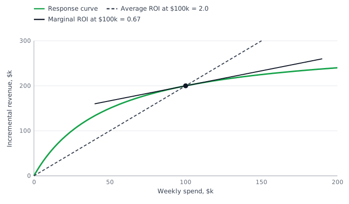
At 100 $k a week, ROI says the channel is excellent: every dollar so far returned two. Marginal ROI says the next dollar returns 67 cents of revenue. Setting mROI to 1 gives the revenue break-even spend:
Above 72.5 $k a week each extra dollar returns less than a dollar of revenue, although average ROI stays well above 1. At 150 $k, ROI is still 1.5 and looks profitable; marginal ROI is 0.375. At 50 $k both metrics say add budget: mROI is 1.5. The two metrics are linked by a simple identity, mROI = ROI × ec / (S + ec); at 100 $k that is 2.0 × 50 / 150 = 0.667. The ratio is the unsaturated share of the curve, so the further a channel is along its curve, the more its average ROI overstates the value of the next dollar. These are revenue ratios: if you decide on gross profit with margin m, the break-even condition is mROI = 1/m, which moves the optimal spend lower.
Budget optimisation scenarios
- Default. Fixed budget. Keeps the total (historical by default) and reallocates it to maximise expected outcome. Each channel is bounded at 70% to 130% of its historical spend unless you change
spend_constraint_lowerandspend_constraint_upper. - Flexible. Target ROI. Finds the largest budget at which total marketing ROI stays at your target. The constraint applies to the total, not to each channel. Default bounds widen to 0% to 200% of historical spend.
- Flexible. Minimum marginal ROI. Lets spend grow while each channel's marginal ROI stays above a floor. This constraint applies per channel, which makes it the closest to the break-even logic above.
All scenarios assume the historical flighting pattern and cost per media unit, optimise the posterior mean of expected outcome, and leave out lagged effects that land after the optimisation window.²⁹ ³⁰ For reach-and-frequency channels the optimiser assumes campaigns run at the optimal frequency unless you set use_optimal_frequency=False.¹⁹
Calibrating Meridian with experiments
From experiment result to ROI prior
Version 2.0 added a calibration builder that turns incrementality results into ROI priors in four steps: register experiments, adjust each one, merge them, and fit a distribution.³¹ A Meridian GeoX result can be registered directly, and the builder reads the point estimate and standard deviation of incremental conversions per dollar (iROAS when the KPI is revenue), the estimated business-as-usual spend and the dates. Any other experiment is registered with its point estimate, standard error, spend and dates.
Each experiment is adjusted before it becomes evidence about the MMM channel:
Here μ and σ are the experiment's point estimate and standard error, the γ terms rescale the estimate and the τ terms inflate the variance; they are calibration factors and have nothing to do with the model's γ (controls) and τ (geo intercepts).³¹ The spend term grows as the experiment's average daily spend departs from the channel's average daily spend in the model window. The duration term divides the estimate of a short test by p, the share of the adstock weight that the test window captured, and widens it by (1 − p)/p; the builder assumes geometric decay with α = 0.5 and a max lag of 8 unless you change it. The recency term uses a 52-week half-life:
Here w is the number of weeks between the experiment's end and the last modelled week. An experiment that ended 52 weeks before the end of the model window gets λ = 0.5 and a recency term of 1, so on its own it widens the standard error by a factor of √2.³¹ Several experiments on one channel are then combined by Bayesian updating:
Here π is an optional baseline prior (flat over positive values if you give none) and N is the number of experiments. The builder evaluates this posterior on a grid and fits a LogNormal, Gamma or Normal distribution to it, which becomes the channel's ROI prior.³¹ The docs are explicit that this is not a precise formula: experiments and MMMs define ROI over different windows, regions and campaign settings, and the prior should carry that extra uncertainty.²²
What 2.0 and 2.1 changed in practice
- 2.0 made calibration a first-class step (the builder plus channel calibration recommendations) and renamed
max_rhattomax_r_hat.⁴ - 2.1 lets you restrict an ROI prior to the experiment's window by channel name and dates (
CalibrationSpec,DateRange) rather than index arrays, and records random holdouts with the saved model. The docs still recommend setting the prior over the full modelling window whenever possible.²⁰ - Caveat for 2.1.0 on JAX. The changelog lists an unreleased fix so that calibrated ROI priors on the JAX backend match TensorFlow. If you calibrate on 2.1.0, plot the resulting priors before fitting.⁴
The estimand trap: heavy-up tests
Meridian GeoX supports three interventions: holdback (new spend in treatment, zero in control), go-dark (existing spend switched off in treatment) and heavy-up (extra spend on top of business as usual), which the GeoX docs position for forecasting the marginal return of more budget.³² The calibration builder is designed for lift measured against a zero-spend counterfactual, and the docs say that registering marginal-lift results is not recommended because of the estimand mismatch.³¹
The geo test in Geo experiments: GeoX and GeoLift is a 4-week heavy-up: 20 $k of extra spend produced 33.2 $k of incremental revenue, an iROAS of 33.2 / 20 = 1.66. That number describes the slope of the curve above current spend, which is closer to marginal ROI than to the channel's average ROI. Registering 1.66 as the ROI prior mixes the two. For an ROI prior, run a go-dark test on an existing channel or a holdback on a new one. A heavy-up result is still useful as a check on the model's marginal ROI, or as input to an mROI prior if you choose that prior type; that last step is my judgement, not a documented recipe.
Running Meridian in Kazakhstan and the CIS
About 20 geos, very unequal
Kazakhstan has 17 oblasts and three cities of republican significance (Almaty, Astana, Shymkent): about 20 geo units, against the 50 to 100 DMAs Google suggests modelling for US advertisers.¹⁵ Two years of weekly data then gives 20 × 104 = 2,080 geo-weeks, and in most consumer businesses Almaty and Astana carry a disproportionate share of the KPI. The docs say the advantage of geo modelling shrinks when there are relatively few geos, and that it is better to model at a finer granularity and drop the smallest geos than to aggregate into coarser regions.¹⁵ With the default single σ, small noisy oblasts can sway the fit; a per-geo σ is available but can make convergence difficult.
What I would do:
- Geo model on oblasts and cities when the KPI and most media spend can be assigned to regions. Drop or merge only the smallest units by KPI, provide official population figures for scaling, and check the EDA population-correlation test. The geo with the largest population becomes the reference by default.
- National model when the KPI cannot be assigned to regions reliably, or most spend is national TV, OOH and Telegram placements without a geo split. Then plan for three years of weekly data, merge channels down to a handful and keep knots few, as in the docs' 26 to 10 parameter example.
- Check the map history. Three oblasts were created in 2022. If your CRM history predates that, map old addresses to the current units before building the table.
Channels, KPI and offline conversions
Search and social platforms usually export spend and impressions by region; check the regional breakdown of each platform you use in Kazakhstan before committing to a geo model. TV, OOH and channel placements in Telegram are typically bought nationally or by city, so the docs' advice applies: impute national media to geos by population share and accept that the model learns less about those channels.²³ Merge channels with low spend rather than estimating each one.
For banks and superapps the KPI that matters (accounts opened, loans disbursed, cards activated) completes in a branch, a call centre or the app. Use that outcome as the KPI, assign it to geos by one consistent rule (client's region or branch region, not a mix), and pass revenue per KPI if you want ROI in money. How to get branch and call-centre outcomes into analytics is covered in Offline attribution for banks; why leads are the wrong KPI when disbursement is the business outcome is in Google Ads leads without disbursements; and the geo-week table itself belongs in your warehouse, see First-party data in a DWH.
Compute
The README recommends at least one GPU and has no official GPU support on macOS; a CPU install works but sampling is slower.⁶ For prototyping, a hosted notebook with a GPU runtime is enough, since Google's own getting-started material is a Colab notebook. For production refits, use a cloud VM with an NVIDIA GPU. The model input is an aggregated geo-week table with no user-level data, which usually makes the compliance conversation shorter than for attribution data, but a bank's security team should still approve where it runs.
Experiments with 20 geos
Geo experiments face the same constraint: with about 20 units and two dominant cities, GeoX's stratified designs have few combinations to choose from, so expect longer tests or larger minimum detectable effects. The options are covered in Geo experiments: GeoX and GeoLift.
Mistakes that cost money
Reading ROI as marginal ROI
"Scale the channel with the best ROI" ranks channels by their average return. In the example above a channel with ROI 2.0 returns 0.667 on the next dollar, and its break-even spend is 72.5 $k a week, not more. Budget moves follow marginal ROI and the response curve.
Default priors on short data
With two years of national data and a dozen channels, the data cannot move the posterior far from LogNormal(0.2, 0.9). The output looks like a measurement but is mostly the prior: every channel lands near the same ROI. Check the prior-posterior plot; channels with no shift need an experiment or a merge, not a presentation.
Skipping the health card
With max R-hat at 1.2 or above, the chains disagree and every downstream number, including the optimiser output, is unreliable. A negative baseline probability above 0.8 means media is over-credited. Fix these before anyone sees a chart.
Moving half the budget at once
Google's measurement playbook recommends adjusting only up to 20% of a channel's spend at a time.³³ Meridian's default fixed-budget bounds are already ±30%. A 50% shift pushes channels into spend levels the model never observed, where the curve is an extrapolation. Move up to 20%, observe, refit, test.
Calibrating ROI with a heavy-up test
A heavy-up measures the return on extra spend above current levels. The calibration builder assumes a zero-spend counterfactual. Use go-dark or holdback tests for ROI priors, and do not let one experiment define a whole channel; the playbook lists that as a pitfall too.³³
Which channel to test first
Take the channel calibration recommendation, sort the flagged channels by spend, and test the largest one whose ROI interval spans 1. That is where an experiment changes the most money.
Next step
The practical next step: build the geo-week table, run Meridian's EDA on it, and list which channels already have an experiment that can serve as an ROI prior.
Sources
¹ Model specification - Meridian, Google for Developers
² Meridian is now available to everyone - Google Blog
³ LightweightMMM README - Google, GitHub
⁴ Meridian CHANGELOG - Google, GitHub
⁵ google-meridian release history - PyPI
⁶ Meridian README - Google, GitHub
⁷ Jin, Wang, Sun, Chan, Koehler (2017). Bayesian Methods for Media Mix Modeling with Carryover and Shape Effects - Google Research
⁸ Sun, Wang, Jin, Chan, Koehler (2017). Geo-level Bayesian Hierarchical Media Mix Modeling - Google Research
⁹ Meridian Scenario Planner - Meridian, Google for Developers
¹⁰ Input data and scaling - Meridian, Google for Developers
¹¹ Default prior distributions - Meridian, Google for Developers
¹² Refresh the model - Meridian, Google for Developers
¹³ Set the adstock_decay_spec parameter - Meridian, Google for Developers
¹⁴ Media saturation and lagging - Meridian, Google for Developers
¹⁵ Geo-level modeling and geo selection - Meridian, Google for Developers
¹⁶ Bayesian inference - Meridian, Google for Developers
¹⁷ Run the model - Meridian, Google for Developers
¹⁸ Reach and frequency - Meridian, Google for Developers
¹⁹ Optimize frequency - Meridian, Google for Developers
²⁰ ROI, mROI and contribution parameterizations - Meridian, Google for Developers
²¹ Choose and configure treatment prior types - Meridian, Google for Developers
²² Calibrate treatment priors - Meridian, Google for Developers
²³ Collect and organize your data - Meridian, Google for Developers
²⁴ Amount of data needed - Meridian, Google for Developers
²⁵ Perform exploratory data analysis - Meridian, Google for Developers
²⁶ Model health checks - Meridian, Google for Developers
²⁷ Channel calibration recommendation and score - Meridian, Google for Developers
²⁸ ROI, mROI and response curves - Meridian, Google for Developers
²⁹ Budget optimization scenarios - Meridian, Google for Developers
³⁰ Optimization without reach and frequency - Meridian, Google for Developers
³¹ Set custom ROI priors using past experiments - Meridian, Google for Developers
³² Types of experiments - Meridian GeoX, Google for Developers
³³ Modern Measurement Playbook (2024) - Think with Google
FAQ
Can we run Meridian without a GPU?
Yes. The CPU install works, and so does macOS, which has no official GPU support; sampling is just slower. The README recommends at least one GPU and says the project was tested on a T4 with 16 GB, so for regular refits of a geo model a GPU runtime saves real time. During exploration, posterior thinning cuts downstream compute, but report only from the full posterior.
Our KPI is accounts opened or loans disbursed, not revenue. Does Meridian still work?
Yes. The KPI only has to add up across regions and weeks. If you pass revenue per KPI, ROI is reported in money; if you do not, Meridian replaces the per-channel ROI prior with a prior on the total contribution of paid media (mean 40%, standard deviation 20%), and an mROI prior then needs a custom distribution.
How often should we refit the model?
Google suggests a cadence that matches your budget decisions, for example quarterly or annually. Append the new weeks to the old data instead of modelling the new period alone, and keep the window around two to three years. Meridian does not make media effectiveness time-varying, so the window is a trade-off: more history lowers variance but can add bias if channels have changed, while dropping old weeks removes that bias at the cost of higher variance. Copying the old posterior into new priors counts the old data twice.
Is Meridian biased towards Google channels?
The model code is open and channel-agnostic: every paid channel gets the same default ROI prior, and you can read the specification and priors yourself. The practical asymmetry is data: the docs point to Google's MMM Data Platform for YouTube reach and frequency, while for other channels you assemble comparable data yourself. Calibrating each major channel with its own experiment is the real protection against bias from any direction.
We already use LightweightMMM. Do we have to migrate?
In practice, yes: the LightweightMMM repository is archived and its README says it is no longer supported. Development continues in Meridian, which is where ROI-parameterised priors, reach and frequency inputs, calibration from experiments and the health card live, and the Meridian README links a migration guide. Expect results to differ, so run both on the same data once and explain the gaps before switching your reporting.
Seeing this in your own funnel?
Two weeks, fixed scope, read-only access. You get the findings and a 90-day roadmap whether or not we work together afterwards.