
Marketing mix modeling (MMM) estimates how much of your sales each channel actually caused, TV and outdoor included, and what the next dollar in each channel is likely to return. It works from aggregated weekly data, with no cookies or user IDs, which is a large part of why it has come back into use. The entry ticket is about two years of clean weekly history in which spend actually moved, and what you get back is an estimate with uncertainty, not proof: it becomes trustworthy only once experiments start checking it.
This is the hub of a four-part series. Here: what MMM is and whether you need it now. Then: Google Meridian in practice, geo experiments with GeoX and GeoLift to validate the model, and Meridian vs Robyn vs PyMC-Marketing to choose a library.
What MMM answers and what it does not
The best short description of the job is still the list of questions in Chan and Perry's 2017 Google paper: what was my return on TV last year, what would sales be if I spent more or less next year, and how should I split the budget to get the most sales.¹ A working MMM gives you four things:
- Incremental contribution per channel. How many sales, applications or how much revenue each channel added on top of a baseline that would have happened anyway. That includes TV, outdoor (OOH), radio and sponsorships, which user-level attribution cannot see at all.
- ROI per channel, computed on that incremental contribution rather than on attributed clicks.
- Response curves. How each channel's contribution changes as its spend goes up or down, so you can see where it saturates.
- Budget scenarios. What happens to the total if money moves between channels, within the range of spend the model has seen.
What it does not do well matters just as much:
| Question | Can MMM answer it? | Better tool |
|---|---|---|
| Which channels added incremental sales last year, TV and OOH included | Yes, this is its core job | - |
| How to split next year's budget across channels | Yes, within the spend range it has seen | Validate large shifts with an experiment |
| Which creative, audience or keyword works better | No: weekly channel totals do not carry that detail | Platform A/B tests, attribution |
| What to change in campaigns this week | No: it is refreshed monthly or quarterly at best | Attribution, platform reporting |
| Proof that channel X caused these sales | Not on its own: it is a regression on historical data | Randomised or geo experiments |
| What happens if we triple a channel's spend | Poorly: that is extrapolation beyond the data | A heavy-up test |
The fifth row is the one teams skip. Chan and Perry point out that MMMs are regressions on a limited amount of observational data, and that their results are correlational rather than causal except under narrow conditions.¹ Google's measurement playbook says the same in practical terms: because MMM rests on correlations, its accuracy depends on the scale, timing and variation of your past spend.² That is not a reason to skip MMM. It is a reason to plan experiments alongside it from day one.
The model in one equation
Most MMMs in use today, Meridian, Robyn and PyMC-Marketing included, share the skeleton that Jin et al. wrote out in a 2017 Google paper:³
Here is the KPI in week t (sales, revenue, approved applications), is the baseline (intercept plus trend and seasonality: what you would sell with no paid media), is the spend or impressions of channel c in week t, Adstock carries part of earlier weeks' media into this week with decay , Hill bends it into diminishing returns with half-saturation point and slope , is the channel's maximum effect, are control variables (price, promotions, holidays, macro, competitors) with coefficients , and is the noise the model does not explain.
Three properties to keep in mind before you read any vendor deck:
- Media effects are additive. Each channel is its own term, which is what lets the model split sales into a baseline plus channels. Jin et al. note that this ignores synergy between channels for simplicity.³
- Carryover first, then saturation is the usual order. Meridian applies Hill to adstocked media unless you switch it,⁴ and Jin et al. explain when the reverse order is better: when spend comes in a few short on-off bursts.³
- Libraries normalise adstock differently. Jin et al., Meridian and PyMC-Marketing (by default) divide the adstock weights by their sum, so adstocked media stays on the scale of spend.³ ⁴ ⁵ Robyn's geometric adstock is the plain recursive sum, which inflates the total by 1/(1-θ).⁶ The same θ therefore means different things in different tools, and β and ec absorb the difference. Compare curves and ROI across models, never raw parameters.
Jin et al. add a second reason to read curves rather than coefficients: quite different combinations of β, ec and s can draw almost the same curve within the observed spend range, so the individual parameters are sometimes close to unidentifiable even when the curve itself is estimated well.³
Adstock: advertising that keeps working after the flight
The idea that advertising builds up and decays, instead of working only in the week it airs, goes back to Simon Broadbent, who introduced the term adstock in his 1979 paper "One Way TV Advertisements Work" in the Journal of the Market Research Society. The simplest and still most common form is geometric decay:
is the adstocked media in week t, is this week's spend, and θ (between 0 and 1) is the share of last week's adstock that survives into this week. This is the unnormalised form Robyn uses; the charts in this series use it because the numbers are easy to follow.
Take a single burst of 100 in week 1 and nothing afterwards:
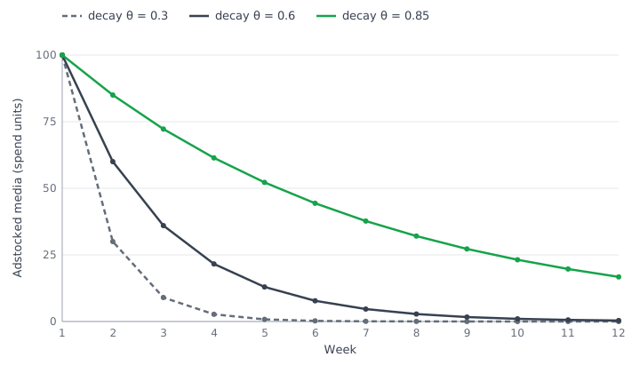
| Week | θ = 0.3 | θ = 0.6 | θ = 0.85 |
|---|---|---|---|
| 1 | 100 | 100 | 100 |
| 2 | 30 | 60 | 85 |
| 3 | 9 | 36 | 72.25 |
| 4 | 2.7 | 21.6 | 61.41 |
| 5 | 0.81 | 12.96 | 52.2 |
| 6 | 0.24 | 7.78 | 44.37 |
| Total, weeks 1-12 | 142.86 | 249.46 | 571.84 |
| Total, all weeks | 142.86 | 250 | 666.67 |
Each week keeps θ of the previous one, so the total effect of the burst is a geometric series:
Here 100 is the burst and k counts the weeks after it: θ = 0.3 gives 100/0.7 = 142.86, θ = 0.6 gives 100/0.4 = 250, θ = 0.85 gives 100/0.15 = 666.67.
Two practical readings. First, a slow channel spreads its effect over months: with θ = 0.85 only 571.84 of the 666.67 has arrived after 12 weeks, so a model with a short lag window, or a test read too early, misses part of it. Second, the decay rate drives how much credit a channel gets for sales that happen weeks after it stopped, which is why it should be estimated, not typed in.
For starting ranges, Robyn's documentation gives a rule of thumb from weekly models its team has built: TV 0.3-0.8, OOH, print and radio 0.1-0.4, digital 0.0-0.3.⁶ Use these as bounds for priors or hyperparameters, not as facts about your market.
Some channels peak late. Geometric decay puts the peak in the week of spend. For media that need time to build, such as a long TV campaign or a brand launch, Jin et al. propose a delayed adstock with a lagged peak, which PyMC-Marketing implements, and Robyn offers Weibull shapes for the same purpose. Check what your library supports before forcing geometric decay on every channel.
Saturation: why the second million buys less than the first
The second transformation captures diminishing returns. The standard form is the Hill function, which Jin et al. borrowed from pharmacology:³
x is the (adstocked) media, ec is the half-saturation point, the level at which the channel delivers half of its maximum effect, and s is the slope that sets the shape; the output runs from 0 to 1 and is multiplied by β to become the channel's effect.
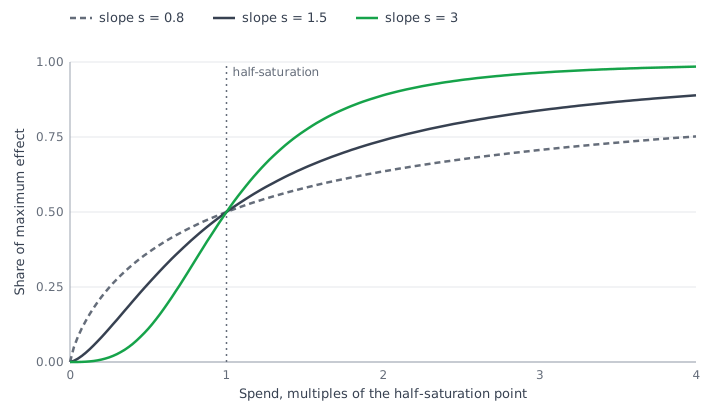
Worked numbers with ec = 100 and s = 1, so Hill(x) = x / (x + 100):
| Spend x | Hill(x) | Calculation |
|---|---|---|
| 50 | 0.333 | 50 / 150 |
| 100 | 0.5 | 100 / 200 |
| 200 | 0.667 | 200 / 300 |
| 400 | 0.8 | 400 / 500 |
Doubling spend from 100 to 200 lifts the effect from 0.5 to 0.667: a third more, not double. Doubling again to 400 adds about a fifth (0.8 / 0.667). That table is the whole case for reallocation: the same dollar is worth more in a channel that still sits on the steep part of its curve.
Two notes from practice. Meridian's default prior assumes a concave curve for paid media, and its documentation warns that S-shaped curves can cause problems for budget optimisation (as of October 2026).⁷ And an S-shape can only be learned if your history contains weeks of low spend: Jin et al. show that when the half-saturation point lies outside the observed spend range, very different curves fit the data equally well.³
From data to decisions: the MMM pipeline
From weekly data to a budget decision
One regression, read three ways, checked by experiments
Weekly data
KPI from the backend
Spend and exposure per channel
Controls: price, promo, season
- 2+ years
Transform and fit
Adstock
Hill saturation
Bayesian or ridge fit
- holdout check
Read
Decomposition
ROI, mROI
Response curves
- intervals, not points
Decide
Budget scenarios
At most 20% per step
Test the biggest bets
- experiments
Experiment results go back into the model as calibration.
The loop repeats when budgets are set, quarterly or yearly.
- Data. Weekly KPI, spend and exposure per channel, control variables. In every MMM project I have seen, this step takes most of the time.
- Transformations. Adstock and saturation per channel, with their parameters estimated from the data rather than set by hand.
- Model fit. Meridian and PyMC-Marketing are Bayesian: you set priors and get a posterior distribution for every parameter. Robyn fits ridge regressions, searches the transformation parameters with an optimiser, and picks among many candidate models on both fit and a plausibility criterion that compares each channel's share of effect with its share of spend.⁶ The comparison article goes through the trade-offs.
- Outputs. Decomposition, ROI and marginal ROI, response curves: next section.
- Budget scenarios. An optimiser moves money between channels along the response curves, within bounds you set.
- Experiments. The channels with the widest uncertainty and the biggest planned shifts get tested, and the results flow back into the model as calibration: priors in a Bayesian model, a calibration objective in Robyn.
Reading the outputs
Check the fit on weeks the model never saw
Before reading any ROI, hold back the most recent weeks and score the model on them. The figure uses a simulated brand with three channels whose true ROI is known: a regression that is given the true adstock and saturation shapes is fitted on 91 weeks and scored on the last 13. In-sample R² is 0.917, and the mean absolute percentage error on the holdout weeks is 7.3%.
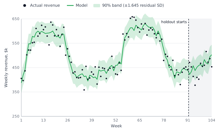
A good holdout score is necessary, not sufficient. On these same data the model cannot separate outdoor from the baseline, because outdoor spend barely moves: its ROI interval stays at 0.29 to 3.52, against 0.28 to 4.69 for the prior alone. The Meridian article shows what that looks like and what one experiment changes.
Decomposition: where the sales came from
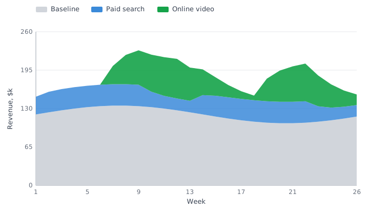
The chart is a synthetic example. Over 26 weeks the model attributes 3,120 to the baseline, 814 to paid search and 858 to online video ($k), 4,792 in total. A channel's share is its contribution divided by the sum:
is the channel's (or the baseline's) modelled revenue over the period and the sum runs over all components, so baseline = 3,120 / 4,792 = 65.1%, paid search = 814 / 4,792 = 17.0%, video = 858 / 4,792 = 17.9%.
Two checks I run on every decomposition before anyone discusses channels:
- Is the baseline plausible? A 65% baseline says that about two thirds of revenue in this window would have happened with no paid media at all. Whether that is believable is a business question: ask sales and finance before you accept it. A baseline that dips below zero in some weeks almost always means the model is misspecified, not that marketing is brilliant.
- What is search getting credit for? Always-on search, brand search above all, follows demand that other channels and the brand created. Chan and Perry name paid search and remarketing as textbook cases of selection bias,¹ and Google's playbook calls search notoriously hard to measure in MMM and recommends testing it regularly.²
ROI and marginal ROI
ROI says how a channel did on average. Marginal ROI (mROI) says what the next dollar will do. Budget decisions run on the second one.
is incremental revenue at weekly spend x, is the most the channel can ever add and ec = 50 is its half-saturation point (all in $k, slope s = 1); ROI is revenue per dollar spent so far, mROI is the derivative, the return on one more dollar.
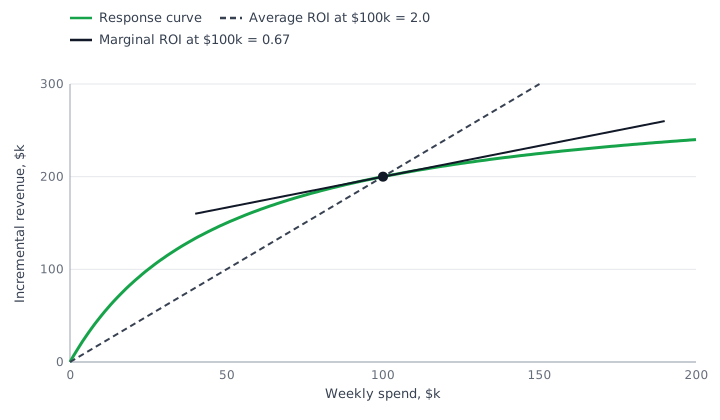
| Weekly spend, $k | Incremental revenue, $k | ROI | mROI |
|---|---|---|---|
| 25 | 100 | 4.0 | 2.667 |
| 50 | 150 | 3.0 | 1.5 |
| 100 | 200 | 2.0 | 0.667 |
| 150 | 225 | 1.5 | 0.375 |
At 50: revenue = 300 × 50 / 100 = 150, ROI = 150 / 50 = 3.0, mROI = 300 × 50 / 100² = 1.5. At 100: revenue = 300 × 100 / 150 = 200, ROI = 2.0, mROI = 15,000 / 150² = 0.667. The point where the next dollar returns exactly one dollar:
Setting mROI to 1 and solving for x gives the break-even spend, here 72.5 ($k per week).
So at $100k a week this channel reports a healthy ROI of 2.0 while every dollar above 72.5 returns less than a dollar. A report that shows only ROI would tell you to keep scaling it. The decision rule is to move money from channels with low mROI to channels with high mROI until marginal returns are roughly equal; Jin et al. formalise the same idea as maximising predicted revenue under a fixed budget.³
Two caveats. MMM ROI includes carryover: Jin et al. count the revenue in the weeks after the spend period as well.³ And the two numbers are not equally reliable: Chan and Perry note that a model can estimate marginal ROI near current spend reasonably well while average ROI stays poor, because average ROI requires extrapolating back to zero spend, a level the data rarely contains.¹
Credible intervals: why a point estimate is dangerous
Every number above is a single point. Real models produce distributions: a posterior in Bayesian models, bootstrap intervals in Robyn. Three reasons never to present the point alone:
- The optimal mix is uncertain too. Jin et al. found that the recommended media mix has a large variance because the parameter estimates do, and that plugging average parameters into the ROI formula can give wrong answers because it ignores how the parameters move together. Compute ROI for every posterior draw, then summarise.³
- Good fit is not validation. In Chan and Perry's example, five plausible models fitted to the same data, all with R² of 0.98-0.99, disagreed on predicted sales by up to 50% and recommended conflicting budget allocations.¹
- Wide intervals tell you what to test next. Google's playbook recommends validating the channels with the widest intervals through incrementality experiments.²
My working rule: show every channel's ROI with its interval. If the interval for a channel spans both "cut it" and "double it", the model has not answered the question for that channel, and that channel is your next experiment.
What you need in place before you start
- 2 years: minimum weekly history (Robyn, Google playbook)
- 3 years: suggested for a national Meridian model
- 10 : 1: observations per model variable (Robyn)
- 4: data points per parameter in Meridian's 104-week example: too few
The sources agree on the floor. Robyn's analyst guide asks for at least two years of weekly data, and more than two years, for example 4-5, if you only have monthly data.⁸ Google's playbook lists at least two years of history as an MMM requirement.² Meridian asks for at least two years of weekly data for geo-level models and three years for national ones, and at least three years if the data is monthly.⁹
Why more is better comes down to counting. Meridian's documentation works through a national model with 12 channels, 6 controls and 8 trend knots: 26 parameters on 104 weekly points is 4 points per parameter, which it calls too low to estimate reliably, and suggests three years (156 / 26 = 6 per parameter) or a geo model.¹⁰ Chan and Perry give 7-10 points per parameter as a rule of thumb for a stable regression and note that modelling lag and saturation takes 3-4 parameters per channel.¹ Robyn's guide recommends about 10 observations per independent variable.⁸
Beyond length, the checklist:
- One KPI, defined the same way for the whole period. If an "application" meant a submitted form in 2024 and an approved application in 2025, the model sees a structural break, not marketing. Meridian also requires a KPI that can be summed across time and regions: units, revenue, conversions, not rates such as CTR.⁹
- A business outcome, not a platform conversion. In banking, insurance and lending the outcome lives in the core system or CRM: approvals, disbursements, policies, often completed offline in a branch or call centre. Bring them into the weekly table; branch attribution and leads without disbursements cover how to capture them.
- Spend and exposure per channel per week, actual rather than planned. Robyn's guide stresses actuals and prefers exposure metrics such as impressions or GRPs where you have them;⁸ Meridian needs spend plus one exposure metric per channel.⁹
- Variation. If a channel's spend barely moved, the model cannot separate its effect from the baseline; Robyn's guide uses the example of TV spend that stays flat while sales vary.⁸ Pauses, flights and regional differences are what the model learns from. Channels that always move together (everything up in Q4) cause the same problem.¹
- Controls. Price and promotions, interest rates for financial products, holidays on the local calendar, product launches, competitor activity, macro indicators.
- A home for the data. A weekly table in your warehouse, rebuilt by a scheduled job, not a spreadsheet someone updates by hand. See first-party data and the DWH. Because MMM uses only aggregated data, cookie loss and consent gaps do not break it the way they break user-level tracking,² as long as the KPI comes from your own backend rather than from platform-reported conversions; the Consent Mode v2 article explains where those gaps come from.
Count parameters before you commission a model. Twenty channels at 3-4 parameters each, plus controls and seasonality, can exceed the 156 points that three years of national weekly data provide. Meridian's documentation lists the remedies: merge small channels, drop near-zero ones, use fewer controls and knots, add years, move to geo-level data, or use stronger priors.
MMM, attribution and experiments: who answers what
| Multi-touch attribution | Incrementality experiments | MMM | |
|---|---|---|---|
| Data | User-level paths (clicks, some views) | Test vs control groups of users or regions | Aggregated weekly totals |
| Measures | Credit for touchpoints on converting paths | Causal incremental effect at one point in time | Modelled incremental contribution over time |
| Channels | Trackable digital | Any channel you can withhold or vary | All, offline included |
| Speed | Daily | Weeks per test | Monthly or quarterly refresh |
| Main weakness | Credits sales that would have happened anyway | Snapshot, costly to scale | Correlational, needs long history |
| Best for | Day-to-day campaign optimisation | Proving and calibrating | Cross-channel budget allocation |
The table follows the overview in Google's playbook.² The same playbook gives a useful way to hold the three together: for digital click-based channels, attribution is usually the generous upper bound, experiments the conservative lower bound, and the MMM estimate should land between them. If it does not, check the setup before arguing about the numbers.
Its rules for combining them are concrete:²
- Compare like with like. The experiment must cover the same channel aggregation and the same metric as the model, and run in a business-as-usual period.
- Gaps of 5-10% between MMM and experiment are acceptable. Below 10% there is no immediate need to recalibrate.
- Above 10%, calibrate the model with the experiment. In a Bayesian MMM the experiment becomes the ROI prior; in a non-Bayesian one the playbook suggests a multiplier, experiment iROAS divided by MMM ROAS.
- Move at most 20% of a channel's spend at a time on MMM forecasts, and validate any change above 10% with an experiment where feasible.
- Do not calibrate a whole channel from a single experiment. Calibrate continuously and across as many channels as possible.
- Do not aim for a single source of truth. Even with a world-class MMM, attribution remains the better tool for day-to-day optimisation.
One experiment, one job. The playbook is explicit that the same experiment cannot both calibrate a model and validate it. If a test result went into the prior, plan a new test to check the refreshed model.
The IAB's December 2025 guidance makes the same case from the advertiser side: integrate MMM with attribution, experimentation and financial systems rather than treating it as a standalone report.¹¹ How to design those experiments, including with few regions, is the subject of the geo experiments article.
When MMM pays off and when it does not
There is no published threshold for "big enough". What follows is my judgement from practice, not a rule from any of the sources.
- Worth it now. Several channels, real history. Four or more channels with meaningful spend, at least one that attribution cannot see (TV, OOH, radio, sponsorship, Telegram placements), two years of weekly data, budgets set quarterly or yearly, and someone with the authority to act on a reallocation.
- Prepare first. Channels yes, data not yet. The KPI changed definition, spend lives in agency spreadsheets, or the outcome is an offline event that is not yet in the warehouse. Spend the next months building the weekly table and running a first experiment.
- Not yet. Too simple or too new. One or two digital channels, where platform experiments and attribution answer the question more cheaply; a business model that changed fundamentally less than two years ago; or spend that has been flat for the whole period.
My test for budget size: take the annual media budget, assume a better allocation improves its efficiency by a modest few percent, and compare that with the yearly cost of the model, meaning data engineering, analyst time, refreshes and one or two experiments. If the first number does not clearly exceed the second, invest in data and experiments first and come back to MMM in a year.
Kazakhstan and the CIS: what changes
Few geo units. Kazakhstan has 17 regions and 3 cities of republican significance (Almaty, Astana, Shymkent), so about 20 geo units.¹² Meridian's documentation illustrates a geo model with 105 geos and 156 weeks.¹⁰ Geo-level models gain precision from many regions and from variation in spend between them,¹³ and with 20 units of very unequal size, Almaty and Astana dwarfing the rest for most consumer brands I work with, that gain is limited. Geo experiments hit the same wall: GeoLift recommends more than 20 geo units,¹⁴ and Kazakhstan sits right at that line.
What I do about it:
- Start with a national weekly model and invest in well-argued priors and experiments rather than geo granularity.
- Go geo-level only when both sides are regional: KPI by region of the customer or branch, and spend that was actually bought by region. Sun et al. show that geo-level estimates deteriorate as more media variables are imputed from national data,¹³ and national TV, Yandex or Telegram campaigns split by population share are exactly that kind of imputation.
- For experiments, use cities where the KPI allows, run longer tests, and use matched markets or synthetic controls rather than a simple random split; treat Almaty and Astana separately instead of letting one of them land alone in the test group. Details in the geo experiments article.
The local channel mix. Google, Meta, TikTok, Yandex, Telegram, OOH and TV are the usual set. The data work differs by channel: TV comes as weekly GRPs from the media agency; Telegram placements bought directly in channels often exist only as invoices and post links, so collect cost and views per post and roll them into weeks; OOH is frequently bought on long flat contracts, which gives the model little variation to learn from.
Offline outcomes in banking and superapps. For banks, insurers and superapps the conversion that matters, an approved loan, a disbursement, an activated card, a signed policy, often happens in a branch, a call centre or inside the app. MMM handles that well because it only needs weekly totals from the core system, but someone has to build that weekly feed. See branch attribution and superapp promotion with Firebase and tROAS.
Common mistakes
Treating brand search as a growth driver
Brand search catches demand that TV, OOH and word of mouth created, so the model can hand it credit that belongs elsewhere. Test search with an experiment before you move money into it on the model's word.
Reallocating on average ROI
A channel with ROI 2.0 can have a marginal ROI of 0.67. Move budget on mROI and response curves; average ROI is for reporting the past.
Trusting one model because the fit is good
Equally well-fitting models can disagree on predicted sales by up to 50%. Look at intervals, compare model variants, and treat a high R² as a minimum, not as validation.
Asking about spend levels the model never saw
Doubling a channel or switching it off is extrapolation. Shift at most 20% of a channel's spend at a time and run a heavy-up or holdout test before larger moves.
Modelling leads instead of business outcomes
Form submissions are easy to collect and easy to inflate. If the business earns money on approvals or disbursements, model those, even if it takes extra work to pull them weekly from the core system.
Next step
If you are deciding now, start by assembling the weekly table for the last two years: KPI, spend and exposure per channel, controls. How far you get in two weeks will tell you more about your readiness than any vendor demo, and when the table exists, the Meridian article picks up from there.
Sources
¹ Challenges and Opportunities in Media Mix Modeling (Chan, Perry, 2017) - Google Research
² Modern Measurement Playbook, 2024 edition - Google
³ Bayesian Methods for Media Mix Modeling with Carryover and Shape Effects (Jin et al., 2017) - Google Research
⁴ Model specification - Meridian, Google for Developers
⁵ GeometricAdstock - PyMC-Marketing API reference
⁶ Features: adstock, saturation and model selection - Robyn, Meta
⁷ Media saturation and lagging - Meridian, Google for Developers
⁸ Analyst's guide to MMM - Robyn, Meta
⁹ Collect and organize your data - Meridian, Google for Developers
¹⁰ Amount of data needed - Meridian, Google for Developers
¹¹ Modernizing MMM: Best Practices for Marketers - IAB
¹² Administrative-territorial units of the Republic of Kazakhstan (July 1, 2023) - Bureau of National Statistics
¹³ Geo-level Bayesian Hierarchical Media Mix Modeling (Sun et al., 2017) - Google Research
¹⁴ GeoLift - Meta, GitHub
FAQ
How long does it take to build a first MMM?
In my experience the modelling is the short part: assembling, cleaning and agreeing on two years of weekly KPI, spend and control data takes most of the calendar time. Once the weekly table exists, a first credible model is a matter of weeks. A geo experiment to validate it adds more: Google's GeoX guidance plans 7-14 weeks end to end, including planning and cool-down.
Can we build an MMM on monthly data?
You can, but you need a longer history: Robyn's guide suggests more than two years, for example 4-5, and Meridian asks for at least three years of monthly data. Monthly data gives 12 points a year instead of 52, so the model can afford far fewer parameters, and Meridian's documentation warns of non-convergence or wide credible intervals. If weekly data exists anywhere, and in ad platforms and core systems it usually does, rebuild the history weekly.
If we have an MMM, do we still need attribution?
Yes. Google's playbook is explicit that even a world-class MMM does not replace attribution for day-to-day optimisation. MMM is refreshed monthly or quarterly at channel level, attribution answers daily at campaign and keyword level. Use MMM and experiments to set budgets between channels, and attribution, ideally calibrated by experiments, to steer inside them.
How often should the model be refreshed?
My default is a refresh with new data every quarter and a full rebuild once a year or after a major change in the business or the channel mix. Between refreshes, move no more than 20% of a channel's spend at a time and keep running experiments so the next refresh has fresh calibration. A refresh that swings a channel's ROI sharply on three new months of data is a warning sign, not news.
Is MMM affected by cookie loss, ITP and consent banners?
Not directly: MMM uses aggregated weekly totals and needs no user-level data, which Google's playbook names as the reason it is more future-proof. The catch is the KPI. If it comes from platform-reported or GA4 conversions, it inherits their consent and tracking gaps, and a change in consent rate looks like a change in sales, so take the KPI from your own backend or core system.
Seeing this in your own funnel?
Two weeks, fixed scope, read-only access. You get the findings and a 90-day roadmap whether or not we work together afterwards.